"Walk Me Through Attention" — By Hand
Article 3 of The AI Engineer Loop — what a 2026 AI Engineer interview actually tests, question by question. Version française.
There is exactly one mechanism inside a transformer you are expected to explain from scratch. Not backprop, not the optimizer, not the tokenizer. Attention.
And the question rarely arrives as "explain attention." It arrives as "walk me through it with actual numbers" — usually after you have given the textbook answer and the interviewer wants to know whether there is anything behind it. Q, K and V. Dot product. Scale by √d_k. Softmax. Weighted sum. Four sentences that anyone can memorise in an afternoon, and which tell an interviewer nothing.
"What does attention actually improve?"
Have an answer to this one before you touch the arithmetic. It is the framing question, and plenty of candidates go straight to the matrices without ever saying what problem those matrices solve.
An embedding, on its own, knows nothing about context. The embedding table is a lookup: one word, one row. The word "bank" has one row, and it is the same row in "the river bank" and in "the bank refused the loan." So a model starts every sentence holding context-free vectors, with every ambiguity in the language still fully intact.
What attention improves is exactly that: it turns context-free vectors into context-dependent ones. Each token goes looking, among the other tokens in the sentence, for whatever disambiguates it — and comes back enriched by what it found. This is the only place in a transformer where tokens see each other at all; the MLP that follows processes each token in isolation.
In the example we are about to compute, "drank" goes in knowing only that it is a past-tense verb. It comes out knowing its subject is cat. Nothing else in the architecture can do that.
And what it improves over what came before: RNNs passed information along the sentence, neighbour to neighbour. Distance was expensive — the signal degraded on the way — and the computation was sequential, so it could not be parallelised during training. Attention connects every pair of tokens directly, however far apart they sit, in a single step, and computes every position at once.
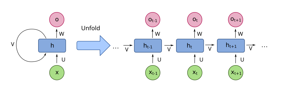
Source: “Recurrent neural network unfold”, fdeloche, Wikimedia Commons, CC BY-SA 4.0 licence. 960 px PNG rendering supplied by Wikimedia, losslessly recompressed (WebP) and hosted on viite.ai; content unchanged. This image remains under CC BY-SA 4.0.

The bill is hidden in "every pair": all pairs get scored, so the cost is O(n²) in sequence length. That is the mechanical reason long context is expensive — and the direct line from this mechanism to your latency budget.
What the question is actually testing
Whether the diagram in your head is a picture or a computation.
The tell is what happens when someone asks why — why divide by √d_k, why every token needs three vectors instead of one, why the output of attention is a blend rather than a choice. If you have done the arithmetic once, those answers are obvious. If you have only read about it, they are three separate things to memorise, and one follow-up question takes you out.
The intuition, before any arithmetic
Q, K and V are three different views of the same token, produced by three learned matrices. The vocabulary is borrowed from information retrieval, which is the fastest way to make it stick.
Think of a library. The query is what this token is looking for. The key is the label another token puts on its spine. The value is what is actually inside the book you pull off the shelf.
Every token produces all three, every time. A token is simultaneously asking for something, advertising what it is, and holding something to hand over.
The setup
Sentence: "the hungry cat drank". Five embedding dimensions, one decimal place, one head of size 2. We compute what the last token, drank, attends to.
The embeddings (d_model = 5)
Real embedding dimensions are not interpretable. Here we pretend they are, so the arithmetic explains itself.
| token | determiner | subject | adjective | verb | past |
|---|---|---|---|---|---|
| the | 0.9 | 0.0 | 0.1 | 0.0 | 0.0 |
| hungry | 0.0 | 0.1 | 0.9 | 0.0 | 0.0 |
| cat | 0.1 | 0.9 | 0.0 | 0.0 | 0.0 |
| drank | 0.0 | 0.1 | 0.0 | 0.9 | 0.8 |
The three learned matrices (5 × 2 each)
These are the weights — the only thing training changes. They ship in the same file as the model itself, the one you download from Hugging Face. Every token in every position uses the same three matrices.
| dimension | W_Q → q1 | q2 | W_K → k1 | k2 | W_V → v1 | v2 |
|---|---|---|---|---|---|---|
| determiner | 0.0 | 0.0 | 0.0 | 0.2 | 0.0 | 0.0 |
| subject | 0.2 | 0.0 | 2.0 | 0.0 | 1.0 | 0.0 |
| adjective | 0.0 | 0.2 | 0.0 | 2.0 | 0.0 | 1.0 |
| verb | 2.0 | 0.4 | 0.2 | 0.0 | 0.1 | 0.1 |
| past | 0.4 | 0.1 | 0.0 | 0.0 | 0.0 | 0.0 |
Read the columns as meanings training landed on. q1 is "I am looking for a subject" — and the verb row is the one that fires it. k1 is "I am a subject" — the subject row fires it. q2 and k2 are the same trick for modifiers. The value columns carry who and what quality.
Step 1 — project "drank" into a query
q = e_drank × W_Q            e_drank = [0.0, 0.1, 0.0, 0.9, 0.8]

q1 of W_Q = [0.0, 0.2, 0.0, 2.0, 0.4]
q2 of W_Q = [0.0, 0.0, 0.2, 0.4, 0.1]

q1 = 0.0(0.0) + 0.1(0.2) + 0.0(0.0) + 0.9(2.0) + 0.8(0.4)
   = 0      + 0.02    + 0      + 1.80    + 0.32   = 2.14
q2 = 0.0(0.0) + 0.1(0.0) + 0.0(0.2) + 0.9(0.4) + 0.8(0.1)
   = 0      + 0       + 0      + 0.36    + 0.08   = 0.44

q(drank) = [2.14, 0.44]
A large first component: the verb is asking loudly for a subject.
Step 2 — project every token into a key and a value
Same arithmetic with W_K and W_V. For cat, e = [0.1, 0.9, 0.0, 0.0, 0.0]:
k1 = 0.1(0.0) + 0.9(2.0) = 1.80        v1 = 0.9(1.0) = 0.90
k2 = 0.1(0.2) + 0.9(0.0) = 0.02        v2 = 0.9(0.0) = 0.00
Across the sentence:
| token | k1 | k2 | v1 (who) | v2 (quality) |
|---|---|---|---|---|
| the | 0.00 | 0.38 | 0.00 | 0.10 |
| hungry | 0.20 | 1.80 | 0.10 | 0.90 |
| cat | 1.80 | 0.02 | 0.90 | 0.00 |
| drank | 0.38 | 0.00 | 0.19 | 0.09 |
Step 3 — score, scale, softmax
Score each token, then normalise — the division exists mainly to keep the softmax off the flat ends of its S-curve, where it stops discriminating and the gradients die.
score = (q · k) / √d_k        d_k = 2, so √d_k ≈ 1.414

the     2.14(0.00) + 0.44(0.38) = 0.167  →  0.167/1.414 = 0.118
hungry  2.14(0.20) + 0.44(1.80) = 1.220  →  1.220/1.414 = 0.863
cat     2.14(1.80) + 0.44(0.02) = 3.861  →  3.861/1.414 = 2.730
drank   2.14(0.38) + 0.44(0.00) = 0.813  →  0.813/1.414 = 0.575

exp(0.118)=1.13   exp(0.863)=2.37   exp(2.730)=15.33   exp(0.575)=1.78
sum = 20.61

weights   the     1.13/20.61 = 0.05
          hungry  2.37/20.61 = 0.12
          cat    15.33/20.61 = 0.74      ← where the mass went
          drank   1.78/20.61 = 0.09      (sums to 1.00)
Note what the exponential did. Before the softmax, cat scored about 3× hungry. After it, cat holds 6× the weight. Softmax does not merely normalise — it sharpens, and that is why the scale factor in front of it matters.
Step 4 — blend the values
out = Σ weight × v

out1 = 0.05(0.00) + 0.12(0.10) + 0.74(0.90) + 0.09(0.19) = 0.70
out2 = 0.05(0.10) + 0.12(0.90) + 0.74(0.00) + 0.09(0.09) = 0.12

attention output for "drank" = [0.70, 0.12]
What just happened. The verb went in knowing only that it was a past-tense verb. It came out carrying 0.70 of who and a trace of quality — it has absorbed cat, faintly flavoured by hungry. That vector is added back into the residual stream, so every layer above now sees a "drank" that knows its subject.
Nothing chose cat. No rule fired. A dot product between two learned projections came out large, and a softmax turned that into three quarters of the attention mass.
Four things this example is hiding
Say these out loud after the walkthrough. They are what turn a recital into a conversation.
Scale. Real d_k is 64–128, not 2, and d_model is in the thousands. The √d_k divisor matters more as it grows: without it, dot products get large, the softmax saturates, and gradients vanish. That is the whole answer to "why divide?" — it is a variance argument, not a convention.
Parallelism. Every token computes its own query at the same time. The four rows above are one matrix multiply, not a loop; drank is only the row we followed. This is why transformers train at scale and RNNs do not.
Multiple heads. This was one head. Run 32 with different W_Q/W_K/W_V and one may track subjects while another tracks adjectives; concatenate the outputs and project back to d_model. A head is not a separate model — in a real checkpoint it is a slice of columns out of the layer's single W_Q.
The mask. drank is last, so nothing was masked. Had we queried from cat, the scores for drank would be set to -inf before the softmax — weight exactly 0. That constraint is what makes next-token training possible over a whole sequence at once.
Say it out loud
Every token projects into a query, a key and a value. Score each pair by query·key, divide by √d_k so the softmax does not saturate, softmax into weights, take the weighted sum of values. Every pair gets scored, so it is O(n²) in sequence length — which is the mechanical reason long context is expensive, and why I treat the context window as a budget I allocate rather than space I fill.
That last clause is the one that lands. It connects the mechanism to a decision you make in production, which is the actual thing being tested.
Red flag: naming the paper and stopping. "Attention Is All You Need, 2017, scaled dot-product attention" is a citation, not an explanation. If you cannot say what a value vector carries or why the division is there, the recital does not count.
Going further
If you would rather see the mechanism than read it:
Video: “Attention in transformers, step-by-step | Deep Learning Chapter 6”, by 3Blue1Brown — Watch on YouTube.
And for the Q, K, V angle — the history of the notation and how the three combine — the video “How to explain Q, K and V of Self Attention in Transformers (BERT)?”, by Discover AI.
Next in The AI Engineer Loop: where W_Q, W_K and W_V actually live in a checkpoint — and why "KV matrices" and "the KV cache" are two completely different objects.
At Viite we simplify business processes with AI, but for humans. We also build Business Studio, an app to run your work and personal life in one place.